Table of Contents
- Trajectory parametrization
- 1. The problem, and how it is decomposed
- 2. Why this exists
- 3. The control stack, and where each limit lives
- 4. How the path is produced
- 5. Platform kinematics
- 6. The parametrization modes
- 7. TOPP-RA
- 8. The constraint set
- 9. Frames: why the bound is body-frame
- 10. Numerics: polygon, not cone
- 11. Deployment and performance
- 12. Reproducing, diagnosing, and what is not verified
Trajectory parametrization
How the velocities along a planned path are assigned, and why.
Scope. ARMAR-7 in its Armar7a configuration, and ARMAR-DE. Concrete values are quoted from a named configuration file throughout; a platform whose parameters are not listed here has not been characterised, whatever its configuration currently contains.
1. The problem, and how it is decomposed
The objective. Minimise the time from receiving a navigation request until the robot stands at the goal, subject to collision-freedom, the platform's velocity limits, the drive's dynamic limits, and two constraints on the robot's heading that have nothing to do with dynamics (below). Note what the objective includes: planning time counts. A plan that takes 5 s to compute has already lost more than almost any refinement of the trajectory can win back.
The heading is a constraint, not a free variable
A platform that is holonomic in principle is not free to point anywhere in practice, and the two reasons are worth stating because neither is recoverable from the code:
- The robot should look where it is going. The head-mounted cameras are what detect humans and unmapped obstacles ahead; a heading that ignores the direction of travel drives the robot into space it cannot see. The laser scanners remain as the backstop — the safety guard is built on them (
safety_guard/LaserBasedProximity.h) — but that is a reactive last resort, and needing it means the camera saw nothing in time. - The robot should arrive already facing the target, and not pivot on approach. The heading is held close to the commanded one within
startGoalDistanceThreshold(1000 mm) of the start and goal. Approaching a table straight-on rather than rotating into place means the objects on it are in view during the approach, so perception has already begun by the time the robot arrives.
These enter the orientation optimizer as its movementDirWeight and priorStart/priorEnd terms. They are genuine requirements traded against time, not incidental smoothing — which is what makes the departure in item 4 below a deliberate compromise rather than an oversight.
This is continuous with the published objective rather than something invented here. In our work (Reister et al., 2022), we set the cost c(·) to "the time spent to complete the current task" (Eq. 1) and state the goal as performing the task "in an efficient way, i.e. as fast as possible" (§III).
Of that work, this package provides only the navigation-related components: the cost model of §IV-A and the generation of the resulting platform trajectory. Placement selection and the manipulation-related costs are implemented elsewhere.
The search already minimises time, not distance
This is worth stating early because the opposite is the natural assumption. We model the permissible speed as a function of obstacle clearance,
and deliberately choose the graph edge weight "to be consistent with the velocity described by Eq. 4":
We state the purpose outright — "to find the **time-optimal** path from a start position to all
possible positions in the map" — in contrast to prior work that "only [considers] the Euclidean
distance as edge weights". Both equations are implemented faithfully (ShortestPathFasterAlgorithm.cpp:271-283 and ObstacleAwareVelocityLimit.cpp:43-53, wired together at SPFA.cpp:238-250), sharing the same three constants. Consequently
so the SPFA cost is proportional to predicted traversal time, exactly, up to a constant factor.
| Paper | Code |
|---|---|
λ | obstacleDistanceWeight |
k | obstacleCostExponent |
d_max | obstacleMaxDistance |
d_o | the costmap value (clearance) |
Values are tuned per task and scene, so they are configuration rather than part of the method.
What each stage fixes for the next
The full problem — a time-optimal, collision-free trajectory in SE(2) under the drive's dynamics — is not solved directly. It is decomposed, and each stage treats the previous stage's output as given:
| Stage | Optimises | Treats as fixed |
|---|---|---|
| grid search | traversal time (above), over positions only | — |
| smoothing | geometric residuals: smoothness, obstacle clearance, tracking, spacing | the homotopy class |
| orientation optimization | angular residuals only (see the README's three objectives) | the positions |
| obstacle-aware velocity | nothing — a direct clearance-to-speed map | the path |
| parametrization | Toppra: time, genuinely optimally. Ramping: nothing, it is a heuristic | the path and the heading profile |
Why decomposing is the right trade
Measured on snug_passage_diagonal with ARMAR-7:
| Stage | |
|---|---|
| grid search | 4.3 ms |
| smoothing | 11.1 ms |
| orientation optimization | 1.8 ms |
| other planner stages | 0.1 ms |
| parametrization (TOPP-RA) | 26.5 ms |
| total planning | 44.4 ms |
| traverse | 14.2 s |
| planning, as a share of request-to-goal | 0.31 % |
Planning is negligible against driving, which is precisely the condition under which decomposing wins. A coupled kinodynamic formulation might shave a little off the traverse, but it costs orders of magnitude more to compute; at seconds of planning it would lose outright against the objective above, since that objective counts the planning.
Where optimality is given up
Each of these is a specific, nameable departure — not a general caveat:
- No rotational cost in the search. The edge weight models linear speed only. Because heading is assigned after the search, turning cost is structurally invisible to it, even though executed speed is capped by
v·|dψ/ds| ≤ maxVel.angular. - No acceleration in the search at all. Torque and command-ramp limits enter only through
Toppra, which is not the default —Rampingis. - The costed path is not the executed path. The search prices a staircase over cell centres; what gets driven is the resampled and smoothed path, whose clearances — and therefore whose permissible speeds — differ. The search is not re-run against them.
- The heading trade-off is made blind to its cost in time. This one is not a mistake but a compromise, and the distinction matters. The perception and approach requirements above are real, and honouring them necessarily costs time — a heading that tracks the direction of travel and settles early is not the heading that would be fastest. The departure is that the optimizer cannot see the price it is paying: every residual has the form
weight · periodicDiff(angle, angle), with no term involving time, velocity or any drive limit, while ‘ψ’(s)bounds speed twice over — through the angular velocity limit, and through the body-frame acceleration boundṡ ≤ √(r/|ψ'|)(§9). So the balance between "see where you are going" and "get there quickly" is set by hand, through weights, rather than by measuring what each degree of heading change costs in seconds. **The default parametrization overwrites the searched profile.**RampingforcescornerVelocityat every corner pastcornerLimitand ramps toboundaryVelocityat the ends — none of which was part of the cost the search minimised.**Geometry and speed are never co-optimised.**Toppra` cannot widen a corner to allow more speed, and there is no feedback from the parametrization back into the path. The only retry loops in the pipeline are collision-driven.
Two qualifications, so the picture is not neater than the code:
- The orientation optimizer's cost function has no temporal term, but its post-processing does:
smoothOrientationsapplies 32 binomial passes explicitly to raise the speed capmaxVel.angular / max|dψ/ds|(OrientationOptimizer.cpp:58-96). It is an open-loop, hand-tuned correction for an effect the objective cannot see. - The decomposition is a choice, not a limitation. An orientation-aware search exists —
AStarWithOrientationover aCostmap3Dwith 72 orientations per cell — and is simply not the default planner.
What is actually guaranteed
Given the path and the heading profile, Toppra's velocity profile is time-optimal under the constraints of §8. That is the only stage in the pipeline with a real optimality guarantee, and its scope is exactly that: optimal for the geometry it was handed, not optimal overall.
A note on replanning
It would be natural to assume the 10 Hz periodic task replans continuously, and that planning cost must therefore fit inside its 100 ms period (replanningUpdatePeriod, server/Navigator.h:100). It does not. The global-replanning block in Navigator::run() is commented out, carrying the note "symbol globalPlanningRequest is not used, so this code is
dead". The only replanning reachable from the periodic task is checkGlobalPathAlternatives(), which is gated on a non-empty set of target alternatives — so it applies after moveToAlternatives, never after a plain moveTo.
Full plans are therefore computed on moveToAbsolute / updateAbsolute and on the alternatives path, always from scratch: no plan is reused or patched. What the periodic task does spend its budget on is updateScene(true) — a full costmap update every cycle, under the same lock, with its own standing TODO that this "will slow down the navigation loop significantly (>1s)".
2. Why this exists
A core::GlobalTrajectory stores one scalar velocity per position:
There is no time axis. duration() recovers one by Riemann-summing 1/v over each segment, but the stored object is a spatial profile, and nothing in the planning pipeline checks whether the base can physically execute it. The planner assigns velocities from obstacle clearance alone; it knows nothing about mass, motor torque, or how fast the drive may change its commanded velocity.
Two consequences follow directly, and both shape everything below.
Zero is a fixed point. The trajectory controller looks up the feedforward velocity at the current position. At the start pose that lookup returns v(s = 0), and the tracking error is also ~0 because the robot is exactly on the trajectory. If the profile starts at rest, the controller commands zero and the robot never leaves the start. This is why GeneralConfig::boundaryVelocity (150 mm/s) exists: it is the floor that breaks the fixed point. Ramping applies it at the endpoints; Toppra applies it to the whole profile, because clamping only the final waypoint turns a sub-millimetre segment into a step of several thousand mm/s².
Nothing upstream bounds acceleration. Following the chain in §3, a commanded wheel speed is the minimum of seven bounds — and only the last one, in the EtherCAT device at 1 kHz, constrains how fast velocity may change. Everything above it constrains velocity only. Closing that gap is what the Toppra parametrization is for.
3. The control stack, and where each limit lives
| Layer | Rate | Limit it enforces |
|---|---|---|
server/Navigator.cpp | 10 Hz | none directly; pushes maxVel or safety-guard limits down |
global_planning/SPFA.cpp | per request | obstacle-aware velocity (four assignment sites, §8.1), maxVel.linear |
algorithms/parametrization/ | per path segment | Ramping: boundaryVelocity, cornerVelocity over rampLength. Toppra: torque, wheel speed, acceleration norm |
server/execution/PlatformControllerExecutor.cpp | 10 Hz | min(safetyGuard, controller config) — without it the safety guard has no effect |
trajectory_control/global/TrajectoryFollowingController.cpp | 100 Hz | twist limits (linear as a norm), angular feedforward cap |
platform_controller/PlatformGlobalTrajectoryController.cpp | 100 Hz / 1 kHz | none; low-pass alpha only |
EtherCAT armar7_omni/joint_controller/Velocity.cpp | 1 kHz | the command ramp — maxVelocity, maxAcceleration, maxDeceleration, coupled across the linear axes |
OmniWheelPlatformKinematics::calcWheelVelocity | 1 kHz | none — pure C⁻¹v, no per-wheel clamp exists |
Two things are worth stating explicitly because they are easy to get wrong:
- The controller applies its limits in the global frame and then rotates into the robot frame. That is harmless only because the linear limit is a norm — a per-axis limit would not survive the rotation.
- If either twist limit is exactly zero,
applyTwistLimitszeroes both. A safety guard that drives the linear limit to zero therefore also stops rotation.
The seven bounds
In order, a commanded speed is the minimum of:
v_max(d)from costmap clearance (planner, per waypoint)generalConfig.maxVel.linear(planner)- the ramp toward
boundaryVelocity/cornerVelocity(parametrization) min(safetyGuard.linear, controller config limit)— 500 mm/s on ARMAR-7× velocityFactor∈ [0, 1] (controller)- the angular feedforward cap, which lowers linear speed when the required yaw rate exceeds the angular limit (ARMAR-7 only)
maxVelocity= 1500 mm/s, andmaxAcceleration= 250 /maxDeceleration= 400 mm/s² on‖dv/dt‖(EtherCAT ramp)
Only step 7 bounds acceleration.
4. How the path is produced
Everything below operates on a path that SPFAImpl::calculatePath has already produced. Its stages run in this order, and two of them matter enough here to be worth stating:
| Stage | What it does |
|---|---|
| grid search | SPFA over the costmap, edge cost combining distance and obstacle proximity |
constructPath / buildTrajectory | cell centres to a GlobalTrajectory — initial velocities from clearance |
resample | to ~200 waypoints, interpolating velocities positionally |
smoothPositions | deforms the path away from the staircase. May be discarded: if the smoothed path is in collision, the unsmoothed grid path is kept |
recomputeVelocities | re-derives velocities, because smoothing moved the positions they were computed for |
recoveryHandling | prepends an escape segment when the robot starts in collision |
optimizeOrientation | assigns the heading ψ(s) at every waypoint |
stitchTrajectory | joins the recovery and main segments |
finalVelocityClamp | re-applies the obstacle-aware limit, reducing only |
Smoothing runs before orientation optimization, and both run after velocities were first assigned. That ordering is the reason there are four separate velocity assignments (§8.1) rather than one: each stage that moves a waypoint invalidates the velocity computed for its old position.
The heading is not derived from the path. optimizeOrientation is a Ceres problem balancing three terms, each encoding a requirement rather than a preference (§1):
| Term | Weight | Requirement it encodes |
|---|---|---|
| align with the direction of travel | movementDirWeight = 0.5 | the cameras must face the space the robot is driving into |
stay near the commanded start / goal heading, within startGoalDistanceThreshold = 1000 mm | priorStartWeight = 0.5, priorEndWeight = 1.0 | arrive facing the target instead of pivoting on the spot, so perception starts during the approach |
| minimise heading change between waypoints | smoothnessWeight = 1.5 | executability — see below |
(Deployed values from config/global_planning/OrientationOptimizer.json, which overrides the struct defaults at every plan.) The goal prior outweighs the start prior 2:1, which is what makes the straight-on approach the firmer of the two.
So on a holonomic base ψ(s) is genuinely an independent degree of freedom, not the path tangent. Two consequences run through the rest of this page: the rotating-frame transport term is large (§9), and the body-frame acceleration bound implies
so a wiggly orientation profile costs speed directly. That is why smoothnessWeight is the largest of the three, and why the smoothing weight is not an aesthetic choice — though note that none of these terms can actually see the time they cost (§1, departure 4).
5. Platform kinematics
Both models come from Simox and are used unchanged; the reparametrization only wraps them and converts units.
5.1 Omni-wheel drive (ARMAR-7)
Three wheels, following Liu, Wu, Zhu & Lew (2003), Omni-Directional Mobile Robot Controller Design by Trajectory Linearization, formula 2.2.2. VirtualRobot::OmniWheelPlatformKinematics exposes C(), the forward model:
C is square, so the inverse model is its matrix inverse — no pseudo-inverse is involved.
| Parameter | Symbol | ARMAR-7 |
|---|---|---|
| body radius | L | 323.0 mm |
| wheel radius | R | 62.5 mm |
| angular position of the first wheel | δ | 30° |
| relative angle (front direction) | α | 60° |
| wheel gear ratio | n | 1.0 |
| inverted wheels | [true, false, false] |
5.2 Mecanum drive (ARMAR-DE)
Four wheels, following Doroftei, Grosu & Spinu (2007), Omnidirectional Mobile Robot — Design and Implementation, formulas 8 and 9. VirtualRobot::MecanumPlatformKinematics exposes both directions explicitly:
with J of shape (3, 4) and J_inv of shape (4, 3). J_inv is supplied by the model; it is not a pseudo-inverse, and J · J_inv = I holds to float precision.
| Parameter | Symbol | ARMAR-DE |
|---|---|---|
| gauge (half lateral spacing) | l₁ | 250.0 mm |
| wheelbase (half longitudinal spacing) | l₂ | 300.0 mm |
| wheel radius | R | 95.0 mm |
Two conventions inherited from Simox, both easy to trip over: y points forwards (the paper uses x), and the wheel order is [left front, right front, rear left, rear right].
5.3 Units
The two models do not agree on wheel units, and this has caused a real bug:
| input | output | |
|---|---|---|
OmniWheelPlatformKinematics::C() | wheel rev/s | mm/s, mm/s, rad/s |
MecanumPlatformKinematics::J() | wheel rad/s | mm/s, mm/s, rad/s |
reparametrization/kinematics.py normalises both to SI (m/s, rad/s) behind PlatformKinematics, dividing the omni model by 2π and scaling the linear rows by 10⁻³. Everything downstream of that interface is SI; everything in the JSON configs and the C++ stack is mm. Constraint limits crossing the boundary are converted at exactly one place, in solver.py.
6. The parametrization modes
Selected by core::GeneralConfig::parametrization. Default is Ramping, which is what deployed configurations get.
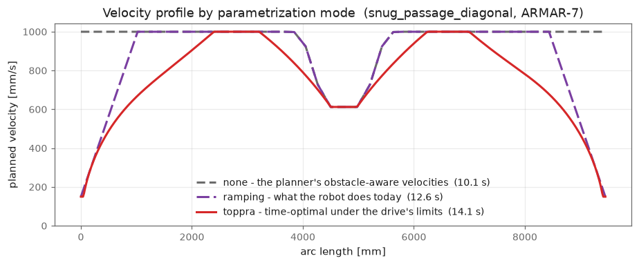
| Mode | What it does |
|---|---|
None | Leaves the planner's obstacle-aware velocities untouched. |
Ramping | Fixes the velocity at the start, the goal and every corner, then interpolates over rampLength. Purely spatial — nothing in it knows about acceleration. |
Toppra | Time-optimal reparametrization under the drive's actual limits (§8). |
A shorter planned duration is not better. In the figure, none is the fastest profile at 10.1 s and also the one the base cannot execute: it plans full speed into the goal and overshoots by ~1.4 m. toppra is the slowest at 14.1 s and reaches the goal with zero overshoot. The planned duration only means something if the profile is executable.
Ramping in detail
GeneralConfig field | Default | Effect |
|---|---|---|
enableRampingStart | true | fixes index 0 to the start velocity |
enableRampingEnd | true | fixes the last index to boundaryVelocity |
enableRampingCorners | true | fixes every corner to cornerVelocity |
cornerLimit | 35° | the angle above which a waypoint counts as a corner |
rampLength | 1000 mm | distance over which the ramp interpolates |
cornerVelocity | 200 mm/s | |
boundaryVelocity | 150 mm/s |
Two properties that matter in practice: the ramp is strictly non-increasing (it takes a min, so overlapping ramps compose safely and ramping can never undo an obstacle-aware reduction), and the ramp denominator is max(totalDistance, rampLength) — so on a segment shorter than rampLength the ramp never reaches full speed and the robot crawls the whole way.
7. TOPP-RA
Time-Optimal Path Parameterization by Reachability Analysis: given a fixed geometric path, find the time-optimal velocity profile subject to velocity and acceleration/torque constraints.
Pham, Hung & Pham, Quang Cuong (2018). A New Approach to Time-Optimal Path Parameterization Based on Reachability Analysis. IEEE Transactions on Robotics 34, 645–659.
The path is parametrised by arc length s, so ṡ is literally the platform's speed. With u = s̈ and x = ṡ², every constraint below is linear in (u, x), which is what makes the problem an LP at each gridpoint.
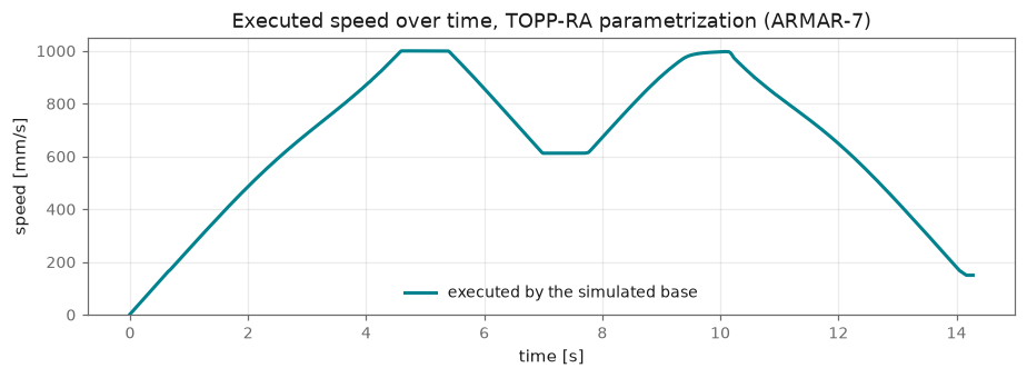
The result is executed by the simulated base with zero goal overshoot and a peak tracking error of a few millimetres.
8. The constraint set
8.1 Obstacle-aware velocity
with d the clearance (obstacle distance minus robot radius), and defaults d_max = 500 mm, w = 2, e = 4. Applied by the planner at four separate points in SPFAImpl::calculatePath (initial assignment, setMaxVelocity, a recompute after position smoothing that overwrites rather than mins, and a final clamp that only reduces), then carried through as the per-waypoint cap the reparametrization must respect.
Two caveats worth knowing:
- Missing costmap data counts as zero clearance, i.e. maximally restrictive. Not knowing how far the obstacles are is not a reason to drive fast.
- These same three parameters are also SPFA's edge-cost parameters, with the proximity term written out identically. The velocity limit cannot be tuned without changing the route. At the default exponent of 4 the limit is within 5 % of maximum already at 299 mm clearance, so it frequently does nothing at all — inspect it with
plot-velocity-limit.
8.2 Angular velocity
|ψ̇| ≤ maxVel.angular, expressed through the same varying velocity constraint: since ‘ψ̇ = ψ’(s)·ṡ, it capsṡ ≤ maxAngular / |ψ'(s)|`.
8.3 Per-wheel speed
The Cartesian cap does not imply a per-wheel one, because wheel rate depends on the direction of travel: a mecanum wheel goes with |v_x| + |v_y|, so a diagonal traverse needs up to √2 times the wheel speed of a straight one at the same Cartesian speed. With ‘ω = J⁻¹ p’(s) ṡ, each wheel capsṡ ≤ ω_max / |[J⁻¹p'(s)]_i|`, and the minimum over wheels is folded into the same bound.
The body twist must be used here, not the world-frame path derivative — J⁻¹ maps a body twist to wheel rates.
8.4 Per-motor torque
Virtual work gives τ = Jᵀw for a body wrench w, so per-motor torque is Jᵀw / (gear · efficiency), bounded in both directions:
This is a SecondOrderConstraint, not JointTorqueConstraint. The latter requires one torque per path coordinate, which a three-wheel drive satisfies by coincidence and a four-wheel mecanum drive does not; here the wrench stays 3-dimensional and the 2N motor bounds live in F w ≤ g, so the wheel count is free.
| ARMAR-7 | ARMAR-DE | |
|---|---|---|
| gear ratio | 16.0 | 40.0 |
| motor max torque | 0.437 N·m | 1.0 N·m |
| gearbox efficiency | 1.0 | 0.9 |
| torque fraction | 1.0 | 0.084 |
| motor nominal speed | 6260 rpm | 4000 rpm |
| gearbox max input speed | 6000 rpm | 8000 rpm |
ARMAR-DE's torqueFraction of 0.084 is a placeholder, chosen to match ARMAR-7's forward acceleration, not derived from a datasheet. See §12.
8.5 Acceleration norm
The device ramp bounds the norm of the commanded velocity change, so the feasible set is a disc. TOPP-RA's stock JointAccelerationConstraint can only express an axis-aligned box, and shrinking a box by √2 so that it implies the disc is the inscribed square — which costs about 9 % of the trajectory duration (§10).
Instead the disc is approximated by an inscribed regular K-gon, K = 32:
The cos(π/K) factor puts the polygon's vertices on the disc rather than outside it, keeping the constraint a sufficient condition. Radius r = min(maxAcceleration, maxDeceleration) — symmetric by choice: the larger deceleration limit is reserved for the reactive safety guard, and the global plan does not spend it. The yaw axis is deliberately left unconstrained; bounding ψ̈ forces the speed to zero at the handful of points where the orientation profile is wiggly, and cost 32 s instead of 15 s when it was tried.
9. Frames: why the bound is body-frame
The ramp limits the change of the commanded body twist — the rotation into the world frame happens after the ramp, and the ramp's internal state is never re-expressed when the robot yaws. Differentiating v_body = Rᵀv_world:
Rᵀ is a rotation, so it cancels in the norm. Bounding ‖a_body‖ therefore needs no per-gridpoint rotation of the polygon — only the coefficient of x changes, from ‘p’'to p'' − ψ'Jp'. Verified against a finite difference ofRᵀv_world` to 1e-10.
This is not the Coriolis term of the equations of motion
The obvious objection — the platform root sits near the COM, so Coriolis and centrifugal effects should be negligible — is correct, and does not apply.
- Dynamic Coriolis/centrifugal is the
q̇ᵀBq̇term in the equations of motion; it depends on mass and COM offset. ARMAR-7's simulated mass matrix hasM[0,2] = −21.6, implying a COM offset of ~116 mm and a centrifugal force of 2.7 N against 46.7 N to accelerate at the limit — 5.8 %. Small, and already handled inside the torque constraint by RBDL. - Rotating-frame transport is the term above. Its magnitude is
|ω||v|, and it contains no mass, no inertia and no COM. Moving the root exactly onto the COM would change it by nothing.
It is large here because the base is holonomic: yaw is a free DoF that the orientation optimizer sets independently of the path. At the worst point of a measured run the commanded yaw rate was 2.6× what the path curvature required, and |ω|v reached 317 mm/s² against a total world-frame acceleration of 137 mm/s². Put plainly: a robot translating straight at 1 m/s while spinning at 0.355 rad/s has zero world-frame acceleration, yet its wheels must continuously change speed, and the ramp sees 354 mm/s². On a differential-drive base the term essentially vanishes, because heading tracks the tangent.
Measured effect. Bounding the world frame left ‖a_body‖ above the limit on 37 % of samples, peaking 31 % over. Bounding the body frame brings that to 0 %, with ‖a_body‖ peaking at 249.9 against the 250 mm/s² radius.
10. Numerics: polygon, not cone
An exact second-order cone is available: cvxpy is installed and a ConicConstraint subclass supplying an arbitrary P gives an exact Euclidean bound, verified at max‖a‖ = 250.000000 against a limit of 250. It is nonetheless not the default.
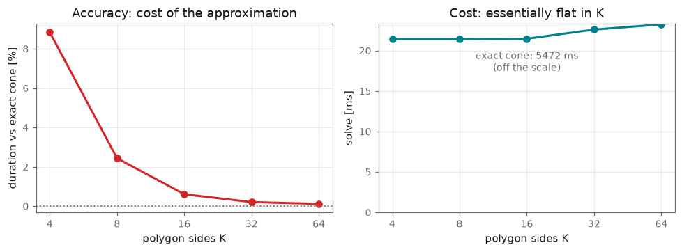
Measured on a 49-waypoint ARMAR-7 path (benchmark-acceleration --exact):
| constraint | duration | vs exact cone | solve |
|---|---|---|---|
| exact cone | 14.664 s | — | 5386 ms |
4-gon (= the old /√2 box) | 15.961 s | +8.84 % | 21.9 ms |
| 8-gon | 15.021 s | +2.43 % | 21.9 ms |
| 16-gon | 14.752 s | +0.60 % | 21.7 ms |
| 32-gon (default) | 14.694 s | +0.20 % | 22.0 ms |
| 64-gon | 14.681 s | +0.11 % | 22.4 ms |
The cone costs 245× the solve time to buy 0.20 % of trajectory duration. Three further reasons it is unsuitable as a default: ConicConstraint hardcodes Collocation, so it would also downgrade the discretization from Interpolation; cvxpy's linear path is broken in this version and returns None on a numerical error, so it is not a general fallback; and upstream C++ toppra has no conic wrapper at all, so the option disappears entirely if this ever migrates to C++.
Solve time is essentially flat in K because the LP solver (seidel) is pinned and handles the extra rows cheaply, which is why K = 32 is free relative to K = 4.
The cone remains reachable — Reparametrizer(acceleration="exact"), and benchmark-acceleration --exact — purely so the polygon has something exact to be measured against.
11. Deployment and performance
Selecting the mode
core::GeneralConfig::parametrization is an enum (None / Ramping / Toppra) with an Aron schema in core/aron/GeneralConfig.xml. A config serialized before the field existed is completed on read with Ramping, not with the enum's zero value — defaulting to None would silently disable ramping on every robot still sending an old config.
Building
The TOPP-RA path needs a python venv and pybind11. CMake derives the interpreter version from the venv rather than naming one, so changing prepare.python.packages[...].python in the Axii module and re-running axii workspace prepare is sufficient; no CMakeLists.txt edit is required. When the venv is missing, configuration still succeeds, logs why TOPP-RA is disabled, and Toppra::apply() throws at runtime with the same reason.
Performance budget
| cost | |
|---|---|
| one-time setup (interpreter, imports, RBDL model) | ~640 ms |
| per navigation request | **~25 ms** (≈20 ms solve, ≈6 ms sampling) |
The setup is paid in Toppra's constructor, i.e. while the navigation stack is being built, not on the first navigation request — the robot is meant to start moving immediately after receiving one.
Trap.
toppra.solverwrapper.available_solvers()probes each wrapper by importing it. Merely havingcvxpyinstalled therefore put ~300 ms ofscipy.statsimport onto the first solve, in a code path that never uses cvxpy. The probe is now forced during construction. If you install theexact-coneextra and see the first request slow down, this is why.
12. Reproducing, diagnosing, and what is not verified
Tools
| Command | Purpose |
|---|---|
plot-planning | Plan on a synthetic scene, simulate execution, plot everything. The main entry point. |
benchmark-acceleration | Regenerate the K-gon table in §10, optionally against the exact cone. |
plot-velocity-limit | Plot the obstacle-aware limit against clearance — use it before concluding the limit "does nothing". |
make-doc-figures | Regenerate every figure on this page. |
Scenes: narrow_passage / narrow_passage_diagonal (tight, smoothing fails at the default gap), snug_passage_diagonal (tight enough to slow the robot, loose enough to smooth — used throughout this page), wide_passage_diagonal, s_corridor (S-shaped, but the robot stays far from obstacles), u_detour (U-shaped, both bends the same way).
Reading the constraint-utilization panel
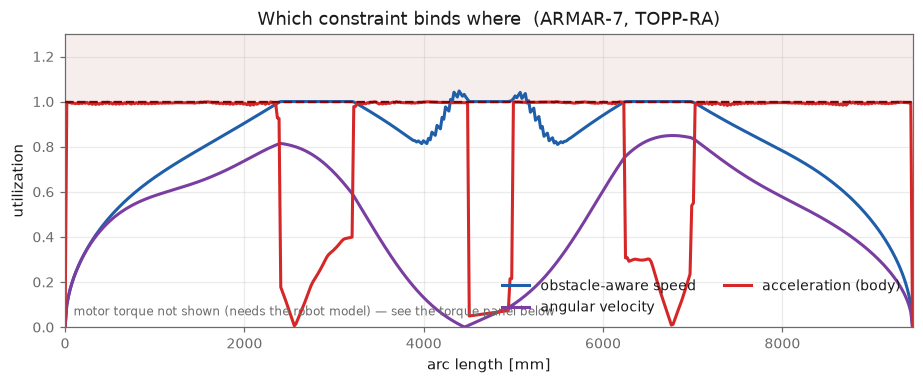
Every constraint normalised to its own bound, so 1.0 means saturated and the binding one is whichever touches the line. This is the panel to look at when the velocity profile dips for no apparent reason — the other panels each plot one quantity against its own limit, and the constraint that actually binds is usually a different one. Motor torque is absent because it needs the RBDL model, which the plotting path does not load; the torque panel covers it.
ARMAR-DE
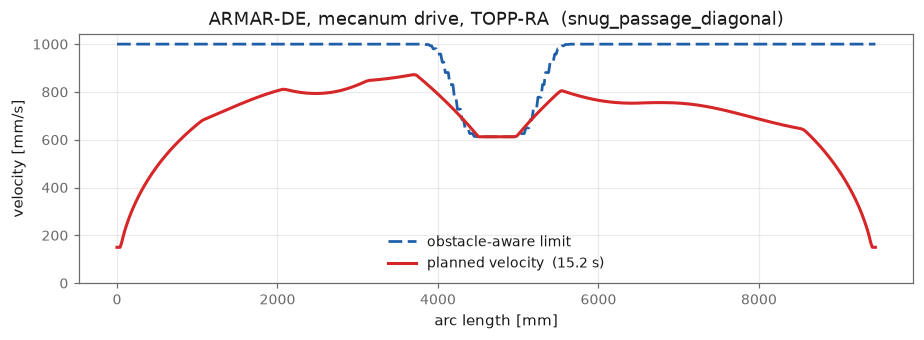
The mecanum path works end to end and produces zero goal overshoot, but the platform's numbers are placeholders. torqueFraction = 0.084 was chosen so its forward acceleration matches ARMAR-7's, not from a datasheet, and it shrinks the torque constraint to 8.4 % of the motor's real capability. Its saturation figures should not be read as a property of the hardware. Its maxLinearAcceleration also equals its ramp limit (both 250 mm/s²), leaving no margin for tracking error, where ARMAR-7 has a factor of two.
Validation status
Verified by measurement:
rampingthrough the parametrization library reproduces the previousNavigator::setupRampingoutput bit-for-bit, andnonereproduces the unparametrized output.- The embedded interpreter produces bit-identical results to the earlier subprocess call.
- Planning is reproducible: repeated runs are bit-identical.
- The body-frame bound is respected on 100 % of samples (§9).
Not verified:
- The
Navigatorpath has never been executed. It compiles, andRampingthrough the factory is bit-identical to the old code via the analysis application — strong evidence, but no test runsNavigator::startGlobalPathSegmentitself. - The python-version switch is verified as a mechanism only; a real second interpreter has not been tried.
Open issues are tracked in BACKLOG.md at the repository root.